UNIT - 1
FUNDAMENTALS OF COMPUTER DESIGN: Introduction; Classes of computers;
Defining computer architecture; Trends in Technology, power in Integrated Circuits and
cost; Dependability; Measuring, reporting and summarizing Performance; Quantitative
Principles of computer design.
6 hours
UNIT - 2
PIPELINING: Introduction; Pipeline hazards; Implementation of pipeline; What makes
pipelining hard to implement?
6 Hours
UNIT - 3
INSTRUCTION –LEVEL PARALLELISM – 1: ILP: Concepts and challenges; Basic
Compiler Techniques for exposing ILP; Reducing Branch costs with prediction;
Overcoming Data hazards with Dynamic scheduling; Hardware-based speculation.
7 Hours
UNIT - 4
INSTRUCTION –LEVEL PARALLELISM – 2: Exploiting ILP using multiple issue
and static scheduling; Exploiting ILP using dynamic scheduling, multiple issue and
speculation; Advanced Techniques for instruction delivery and Speculation; The Intel
Pentium 4 as example. 7 Hours
PART - B
UNIT - 5
MULTIPROCESSORS AND THREAD –LEVEL PARALLELISM: Introduction;
Symmetric shared-memory architectures; Performance of symmetric shared–memory
Advanced Computer Architecture 06CS81
Dept of CSE,SJBIT,Bangalore 2
multiprocessors; Distributed shared memory and directory-based coherence; Basics of
synchronization; Models of Memory Consistency.
7 Hours
UNIT - 6
REVIEW OF MEMORY HIERARCHY: Introduction; Cache performance; Cache
Optimizations, Virtual memory.
6 Hours
UNIT - 7
MEMORY HIERARCHY DESIGN: Introduction; Advanced optimizations of Cache
performance; Memory technology and optimizations; Protection: Virtual memory and
virtual machines.
6 Hours
UNIT - 8
HARDWARE AND SOFTWARE FOR VLIW AND EPIC: Introduction: Exploiting
Instruction-Level Parallelism Statically; Detecting and Enhancing Loop-Level
Parallelism; Scheduling and Structuring Code for Parallelism; Hardware Support for
Exposing Parallelism: Predicated Instructions; Hardware Support for Compiler
Speculation; The Intel IA-64 Architecture and Itanium Processor; Conclusions.
7 Hours
TEXT BOOK:
1. Computer Architecture, A Quantitative Approach – John L. Hennessey and
David A. Patterson:, 4
th Edition, Elsevier, 2007.
REFERENCE BOOKS:
1. Advanced Computer Architecture Parallelism, Scalability – Kai Hwang:,
Programability, Tata Mc Grawhill, 2003.
2. Parallel Computer Architecture, A Hardware / Software Approach – David
E. Culler, Jaswinder Pal Singh, Anoop Gupta:, Morgan Kaufman, 1999.
unit 1 notes:
UNIT I
FUNDAMENTALS OF COMPUTER DESIGN
Introduction
Today’ s desktop computers (less than $500 cost) ar e having more
performance, larger memory and storage than a computer bought in 1085 for 1
million dollar. Highest performance microprocessors of today outperform
Supercomputers of less than 10 years ago. The rapid improvement has come both
from advances in the technology used to build computers and innovations made in
the computer design or in other words, the improvement made in the computers
can be attributed to innovations of technology and architecture design.
During the first 25 years of electronic computers, both forces made a
major contribution, delivering performance improvement of about 25% per year.
Microprocessors were evolved during late 1970s and their ability along with
improvements made in the Integrated Circuit (IC) technology y contributed to 35%
performance growth per year.
The virtual elimination of assembly language programming reduced the n eed
for object-code compatibility. The creation of standardized vendor-independent
operating system lowered the cost and risk of bringing out a new architecture.
In the yearly 1980s, the Reduced Instruction Set Computer (RISC) based
machines focused the attention of designers on two critical performance techniques,
the exploitation Instruction Level Parallelism (ILP) and the use of caches. The figu
re 1.1 shows the growth in processor performance since the mid 1980s. The graph
plots performance relative to the VAX-11/780 as measured b y the SPECint
benchmarks. From the figure it is clear that architectural and organizational
enhancements led to 16 years of sustained growth in performance at an annual rate of
over 50%. Since 2002, processor performance improvement has dropped to about 20%
per year due to the following hurdles:
•Maximum power dissipation of air-cooled chips
•Little ILP left to exploit efficiently
•Limitations laid by memory latency
The hurdles signals historic switch from relying solely on ILP to Thread Level
Parallelism (TLP) and Data Level Parallelism (DLP).
Advanced Computer Architecture 06CS81
Dept of CSE,SJBIT,Bangalore 6
Figure 1.1 The evolution of various classes of computers:
Classes of Computers
1960: Large Main frames (Millions of $ )
(Applications: Business Data processing, large Scientific computin g)
1970: Minicomputers (Scientific laboratories, Time sharing concepts)
1980: Desktop Computers (µPs) in the form of Personal computers and workstations.
(Larger Memory, more computing power, Replaced Time sharing g systems)
1990: Emergence of Internet and WWW, PDAs, emergence of high performance digital
consumer electronics
2000: Cell phones
These changes in computer use have led to three different computing classes each
characterized by different applications, requirements and computing technologies.owth in
processor performance since 1980s
Advanced Computer Architecture 06CS81
Dept of CSE,SJBIT,Bangalore 7
Desktop computing
The first and still the largest market in dollar terms is desktop computing. Desktop
computing system cost range from $ 500 (low end) to $ 5000 (high-end
configuration). Throughout this range in price, the desktop market tends to drive to
optimize price- performance. The perf ormance concerned is compute performance
and graphics performance. The combination of performance and price are the
driving factors to the customers and the computer designer. Hence, the newest,
high performance and cost effective processor often appears first in desktop computers.
Servers:
Servers provide large-scale and reliable computing and file services and are
mainly used in the large-scale en terprise computing and web based services. The three
important
characteristics of servers are:
•Dependability: Severs must operate 24x7 hours a week. Failure of server system
is far more catastrophic than a failure of desktop. Enterprise will lose revenue if
the server is unavailable.
•Scalability: as the business grows, the server may have to provide more
functionality/ services. Thus ability to scale up the computin g capacity, memory,
storage and I/O bandwidth is crucial.
•Throughput: transactions completed per minute or web pages served per second
are crucial for servers.
Embedded Computers
Simple embedded microprocessors are seen in washing machines, printers,
network switches, handheld devices such as cell phones, smart cards video game
devices etc. embedded computers have the widest spread of processing power and
cost. The primary goal is often meeting the performance need at a minimum price
rather than achieving higher performance at a higher price. The other two characteristic
requirements are to minimize the memory and power.
In many embedded applications, the memory can be substantial portion of
the systems cost and it is very important to optimize the memory size in such
cases. The application is expected to fit totally in the memory on the p rocessor
chip or off chip memory. The importance of memory size translates to an emphasis
on code size which is dictated by the application. Larger memory consumes more
power. All these aspects are considered while choosing or designing processor for the
embedded applications.
Advanced Computer Architecture 06CS81
Dept of CSE,SJBIT,Bangalore 8
Defining C omputer Arch itecture
The computer designer has to ascertain the attributes that are important for a
new computer and design the system to maximize the performance while staying
within cost, power and availability constraints. The task has few important aspects such
as Instruction Set design, Functional organization, Logic design and implementation.
Instruction Set Architecture (ISA)
ISA refers to the actual programmer visible Instruction set. The ISA serves as
boundary between the software and hardware. Th e seven dimensions of the ISA are:
i)Class of ISA: Nearly all ISAs today ar e classified as General-PurposeRegister
architectures. The operands are either Registers or Memory locations.
The two popular versions of this class are:
Register-Memory ISAs : ISA of 80x86, can access memory as part of many
instructions.
Load -Store ISA Eg. ISA of MIPS, can access memory only with Load or
Store instructions.
ii)Memory addressing: Byte addressing scheme is most widely used in all
desktop and server computers. Both 80x86 and MIPS use byte addressing.
Incase of MIPS the object must be aligned. An access to an object of s b yte at
byte address A is aligned if A mod s =0. 80x86 does not require alignment.
Accesses are faster if operands are aligned.
iii) Addressing modes:Specify the address of a M object apart from register and constant
operands.
MIPS Addressing modes:
•Register mode addressing
•Immediate mode addressing
•Displacement mode addressing
80x86 in addition to the above addressing modes supports the additional
modes of addressing:
i. Register Indirect
ii. Indexed
iii,Based with Scaled index
iv)Types and sizes of operands:
MIPS and x86 support:
•8 bit (ASCII character), 16 bit(Unicode character)
•32 bit (Integer/word )
•64 bit (long integer/ Double word)
•32 bit (IEEE-754 floating point)
•64 bit (Double precision floating point)
•80x86 also supports 80 bit floating point operand.(extended double
Precision
Advanced Computer Architecture 06CS81
Dept of CSE,SJBIT,Bangalore 9
v)Operations:The general category o f operations are:
oData Transfer
oArithmetic operations
oLogic operations
oControl operations
oMIPS ISA: simple & easy to implement
ox86 ISA: richer & larger set of operations
vi) Control flow instructions:All ISAs support:
Conditional & Unconditional Branches
Procedure C alls & Returns MIPS 80x86
• Conditional Branches tests content of Register Condition code bits
• Procedure C all JAL CALLF
• Return Address in a R Stack in M
vii) Encoding an ISA
Fixed Length ISA Variable Length ISA
MIPS 32 Bit long 80x86 (1-18 bytes)
Simplifies decoding Takes less space
Number of Registers and number of Addressing modes hav e significant
impact on the length of instruction as the register field and addressing mode field
can appear many times in a single instruction.
Trends in Technology
The designer must be aware of the following rapid changes in implementation
technology.
•Integrated C ircuit (IC) Logic technology
•Memory technology (semiconductor DRAM technology)
•Storage o r magnetic disk technology
•Network technology
IC Logic technology:
Transistor density increases by about 35%per year. Increase in die size
corresponds to about 10 % to 20% per year. The combined effect is a growth rate
in transistor count on a chip of about 40% to 55% per year. Semiconductor DRAM
technology:cap acity increases by about 40% per year.
Storage Technology:
Before 1990: the storage density increased by about 30% per year.
After 1990: the storage density increased by about 60 % per year.
Disks are still 50 to 100 times cheaper per bit than DRAM.
Advanced Computer Architecture 06CS81
Dept of CSE,SJBIT,Bangalore 10
Network Technology:
Network performance depends both on the per formance of the switches and
on the performance of the transmission system. Although the technology improves
continuously, the impact of these improvements can be in discrete leaps.
Performance trends: Bandwidth or throughput is the total amount of work done in
given time.
Latency or response time is the time between the start and the completion of an
event. (for eg. Millisecond for disk access)
A simple rule of thumb is that bandwidth gro ws by at least the square of the
improvement in latency. Computer designers should make plans accordingly.
•IC Processes are characterizes by the f ature sizes.
•Feature sizes decreased from 10 microns(1971) to 0.09 microns(2006)
•Feature sizes shrink, devices shrink quadr atically.
•Shrink in vertical direction makes the operating v oltage of the transistor to
reduce.
•Transistor performance improves linearly with decreasing
feature size
Advanced Computer Architecture 06CS81
Dept of CSE,SJBIT,Bangalore 11
.
•Transistor count improves quadratically with a linear improvement in Transistor
performance.
•!!! Wire delay scales poo rly comp ared to Transistor performance.
•Feature sizes shrink, wires get shorter.
•Signal delay fo r a wire increases in proportion to the product of Resistance and
Capacitance.
Trends in Power in Integrated Circuits
For CMOS chips, the dominant source of energy consumption is due to switching
transistor, also called as Dynamic power and is given b y the following equation.
Power = (1/2)*Capacitive load* Voltage
* Frequency switched dynamic
•For mobile devices, energy is the better metric
Energy dynamic = Capacitive load x Voltage 2
•For a fix ed task, slowing clock rate (frequency switched) reduces power, but not energy
•Capacitive load a function of number of transistors connected to output and technology,
which determines capacitance of wires and transistors
•Dropping voltage helps both, so went from 5V down to 1V
•To save energy & dynamic power, most CPUs now turn off clock of inactive modules
•Distributing the power, removing the heat and preventing hot spots have become
increasingly difficult challenges.
• The leakage current flows even when a transistor is off. Therefore static power is
equally important.
Power static= Current static * Voltage
•Leakage current increases in processors with smaller transistor sizes
•Increasing the number of transistors increases power even if they are turned off
•In 2006, goal for leakage is 25% of total power consumption; high performance designs
at 40%
•Very low power systems even gate voltage to inactive modules to control loss due to
leakage
Trends in Cost
• The underlying principle that drives the cost down is the learning curvemanufacturing
costs decrease over time.
• Volume is a second key factor in determining cost. Volume decreases cost since it
increases purchasing manufacturing efficiency. As a rule of thumb, the cost decreases
Advanced Computer Architecture 06CS81
Dept of CSE,SJBIT,Bangalore 12
about 10% for each doubling of volume.
• Cost of an Integrated Circuit
Although the cost of ICs have dropped exponentially, the basic process of silicon
manufacture is unchanged. A wafer is still tested and chopped into dies that are
packaged.
Cost of IC = Cost of [die+ testing die+ Packaging and final test] / (Final test yoeld)
Cost of die = Cost of wafer/ (Die per wafer x Die yield)
The number of dies per wafer is approximately the area of the wafer divided by the area
of the die.
Die per wafer = [_ * (Wafer Dia/2)2/Die area]-[_* wafer dia/_(2*Die area)]
The first term is the ratio of wafer area to die area and the second term compensates for
the rectangular dies near the periphery of round wafers(as shown in figure).
Dependability:
The Infrastructure providers offer Service Level Agreement (SLA) or Service
Level Objectives (SLO) to guarantee that their networking or power services would be
dependable.
Advanced Computer Architecture 06CS81
Dept of CSE,SJBIT,Bangalore 13
• Systems alternate between 2 states of service with respect to an SLA:
1. Service accomplishment, where the service is delivered as specified in SLA
2. Service interruption, where the delivered service is different from the SLA
• Failure = transition from state 1 to state 2
• Restoration = transition from state 2 to state 1
The two main measures of Dependability are Module Reliability and Module
Availability. Module reliability is a measure of continuous service accomplishment (or
time to failure) from a reference initial instant.
1. Mean Time To Failure (MTTF) measures Reliability
2. Failures In Time (FIT) = 1/MTTF, the rate of failures
• Traditionally reported as failures per billion hours of operation
• Mean Time To Repair (MTTR) measures Service Interruption
– Mean Time Between Failures (MTBF) = MTTF+MTTR
• Module availability measures service as alternate between the 2 states of
accomplishment and interruption (number between 0 and 1, e.g. 0.9)
• Module availability = MTTF / ( MTTF + MTTR)
Performance:
The Execution time or Response time is defined as the time between the start and
completion of an event. The total amount of work done in a given time is defined as the
Throughput.
The Administrator of a data center may be interested in increasing the
Throughput. The computer user may be interested in reducing the Response time.
Computer user says that computer is faster when a program runs in less time.
The routinely executed programs are the best candidates for evaluating the performance
of the new computers. To evaluate new system the user would simply compare the
execution time of their workloads.
Benchmarks
Advanced Computer Architecture 06CS81
Dept of CSE,SJBIT,Bangalore 14
The real applications are the best choice of benchmarks to evaluate the
performance. However, for many of the cases, the workloads will not be known at the
time of evaluation. Hence, the benchmark program which resemble the real applications
are chosen. The three types of benchmarks are:
• KERNELS, which are small, key pieces of real applications;
• Toy Programs: which are 100 line programs from beginning programming
assignments, such Quicksort etc.,
• Synthetic Benchmarks: Fake programs invented to try to match the profile and
behavior of real applications such as Dhrystone.
To make the process of evaluation a fair justice, the following points are to be followed.
• Source code modifications are not allowed.
• Source code modifications are allowed, but are essentially impossible.
• Source code modifications are allowed, as long as the modified version produces
the same output.
• To increase predictability, collections of benchmark applications, called
benchmark suites, are popular
• SPECCPU: popular desktop benchmark suite given by Standard Performance
Evaluation committee (SPEC)
– CPU only, split between integer and floating point programs
– SPECint2000 has 12 integer, SPECfp2000 has 14 integer programs
– SPECCPU2006 announced in Spring 2006.
SPECSFS (NFS file server) and SPECWeb (WebServer) added as server
benchmarks
• Transaction Processing Council measures server performance and
costperformance for databases
– TPC-C Complex query for Online Transaction Processing
– TPC-H models ad hoc decision support
– TPC-W a transactional web benchmark
– TPC-App application server and web services benchmark
• SPEC Ratio: Normalize execution times to reference computer, yielding a ratio
proportional to performance = time on reference computer/time on computer being rated
• If program SPECRatio on Computer A is 1.25 times bigger than Computer B, then
Advanced Computer Architecture 06CS81
Dept of CSE,SJBIT,Bangalore 15
• Note : when comparing 2 computers as a ratio, execution times on the reference
computer drop out, so choice of reference computer is irrelevant.
Quantitative Principles of Computer Design
While designing the computer, the advantage of the following points can be
exploited to enhance the performance.
* Parallelism: is one of most important methods for improving performance.
- One of the simplest ways to do this is through pipelining ie, to over lap the
instruction Execution to reduce the total time to complete an instruction
sequence.
- Parallelism can also be exploited at the level of detailed digital design.
- Set- associative caches use multiple banks of memory that are typically searched
n parallel. Carry look ahead which uses parallelism to speed the process of
computing.
* Principle of locality: program tends to reuse data and instructions they have used
recently. The rule of thumb is that program spends 90 % of its execution time in only
10% of the code. With reasonable good accuracy, prediction can be made to find what
instruction and data the program will use in the near future based on its accesses in the
recent past.
* Focus on the common case while making a design trade off, favor the frequent case
over the infrequent case. This principle applies when determining how to spend
resources, since the impact of the improvement is higher if the occurrence is frequent.
Amdahl’s Law: Amdahl’s law is used to find the performance gain that can be obtained
by improving some portion or a functional unit of a computer Amdahl’s law defines the
speedup that can be gained by using a particular feature.
Speedup is the ratio of performance for entire task without using the enhancement
when possible to the performance for entire task without using the enhancement.
Execution time is the reciprocal of performance. Alternatively, speedup is defined as thee
ratio of execution time for entire task without using the enhancement to the execution
time for entair task using the enhancement when possible.
Speedup from some enhancement depends an two factors:
Advanced Computer Architecture 06CS81
Dept of CSE,SJBIT,Bangalore 16
i. The fraction of the computation time in the original computer that can be
converted to take advantage of the enhancement. Fraction enhanced is always less than or
equal to
Example: If 15 seconds of the execution time of a program that takes 50
seconds in total can use an enhancement, the fraction is 15/50 or 0.3
ii. The improvement gained by the enhanced execution mode; ie how much
faster the task would run if the enhanced mode were used for the entire program. Speedup
enhanced is the time of the original mode over the time of the enhanced mode and is always
greater then 1.
The Processor performance Equation:
Processor is connected with a clock running at constant rate. These discrete time events
are called clock ticks or clock cycle.
CPU time for a program can be evaluated:
Advanced Computer Architecture 06CS81
Dept of CSE,SJBIT,Bangalore 17
Example:
A System contains Floating point (FP) and Floating Point Square Root (FPSQR) unit.
FPSQR is responsible for 20% of the execution time. One proposal is to enhance the
FPSQR hardware and speedup this operation by a factor of 15 second alternate is just to
try to make all FP instructions run faster by a factor of 1.6 times faster with the same
effort as required for the fast FPSQR, compare the two design alternative
Advanced Computer Architecture 06CS81
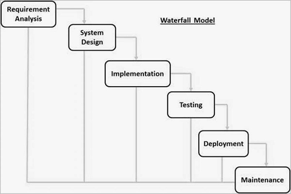 The sequential phases in Waterfall model are: